Recently, there has been much discussion in the press and media about changes to the global climate system, particularly in relation to the increasing number of severe hurricanes and typhoons and the increasing number of extreme rainfall events that lead to catastrophic flooding. It is said that various tipping points in the climate system have been passed. But what exactly is a tipping point?
The dictionary definition of a tipping point is that critical point in a situation, process, or system beyond which a significant and often unstoppable effect or change takes place.
The models of the climate system are very complex, with many parameters and variables. An understanding of the mathematical details of these models requires specialized training.
However, I will illustrate here the concept of a tipping point using a model based on the logistic equation. This is the simplest complex model having only single parameter, R, and a single variable, x.
Like all models, this model evolves from one state to the next. At any point in time, the value of the only variable, x, defines the state of the system that time. The value of the variable at any stage also uniquely defines the value of the variable in the next stage in the evolution of the system.
The fixed value of the only parameter, R, defines the behaviour of the model and the value of that parameter if fixed within each model.
The Excel spreadsheet used in this video can be downloaded from my Google drive, so that you can play and have fun with the The Model.
https://docs.google.com/spreadsheets/d/1UKL7Xs_JOFzF0QxQwO7vMwe0ZDMAw3zN/edit?usp=sharing&ouid=102006032652758740566&rtpof=true&sd=true
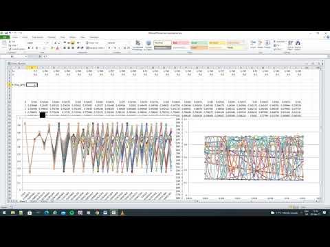
The spreadsheet contains a number of models, 25 in all, each contained within its own vertical column, B to Z. The models in the different columns differ from each other in that the value of the parameter, R, used in the models increases slightly for each model across the spreadsheet. This allows for rapid visual inspection of the differences in the behaviour and evolution of each model.
The two graphs show the evolution of the models from differing points of view. The graph on the left shows how the values of the variable change going down the column. Thus, each model is represented as a single line. On the other hand, the graph on the right shows how the values of the variable in the different models change, either in near sync with each other, showing as almost horizontal lines or as a set of more complicated curves if there is a significant divergence in the evolution of the variables between the models.
As I said before, each of the 25 models on the Excel spreadsheet is contained in its own single column. The model in column B has a parameter value R = 0.4. The model in column Z has a parameter value R = 0.424. Models in the intervening columns have parameter values between these two values.
Looking at the left hand graph, it is clear that the state of each model (i.e. the values of the variable x) decay rapidly along a similar path to zero.
The right hand graph shows that there is the changes in each model are in close agreement with each other.
We are now in a position to explore a wide range of values for the parameter R and see who these alter the behaviour and evolution nature of each model.
This is my illustration of tipping points:
(a) monotonic closure to an asymptote state,
(b) a ringing closure on an asymptote state,
(c) oscillation between well-defined stable states,
(d) oscillation between bands of states,
(e) chaotic ill-defined states.
This model has nothing to do with the climate system. In a climate model there are multiple parameters and a huge number of variables.


0 Comments